Planning

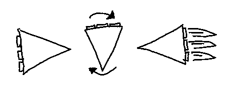
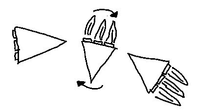
For a quite a while, I have wanted to try and create simple touch based interface for a 2D spaceship game. I want to allow the player to simply drag anywhere on the screen, and the spaceship moves to that position and direction in an efficient manner. Ideally the most efficient manner.

Spaceships in 2D games usually have one main engine that allows forward thrust, and some that allow rotation around the ships center of mass.

Moving from point A to B efficiently (in minimal time) is not trivial with such constraints, as changes to direction and thrust may have huge consequences for later possible movements due to inertia.

So instead of looking at the full A to B problem immediately, I wanted to look at something simpler first, namely to go from having velocity $v_0$ and pointing in direction $\theta_0$ to have 0 velocity as fast as possible.

The idea I use originally came from talking to a colleague, but something very similar sounding is mentioned in planning algorithms, though examples always seems to involve driftless systems. Anyway, my current approach involves these known quantities and assumptions:

$a$ – Acceleration – The ship can only accelerate by a constant amount, and acceleration turns on and off instantly.
$s$ – Turn speed – rotating the ship requires no acceleration, and the ship has constant rotation rate.
$\theta_0$ – Initial orientation.
$v_0$ – Initial velocity

These quantities allow me to find a legal, but very suboptimal way to stop. It simply involves to turn the ship to face its velocity vector, and then accelerate until it stops. Both the time needed to turn the ship $t_a$ and the time $t_m$ needed to turn and reverse the velocity are easy to calculate.

Turn until facing velocity and initiate burn at time $t_a$. At $t_m$ the ship has velocity 0.

It is also easy to see that this is suboptimal, it would clearly be faster, to start burning some time before the turn is fully completed, but the question is when to start the burn.

To allow for this freedom in my model, I therefore introduce a third time variable $t_s$. $t_s$ is the time to start turning and accelerating at the same time. $t_a$ now becomes the time when I stop turning and only accelerate.

Turn and initiate burn after $t_s$ time, at $t_a$ time only accelerate. At $t_m$ the ship has velocity 0.

Given these intervals, two integrals describe how the velocity will change when $t_s$, $t_a$ and $t_m$ vary.

$$ v_x = \int_{t_s}^{t_a} a\cos(\theta_0+st)dt + \int_{t_a}^{t_m} a\cos(\theta_0+st_a)dt $$

$$ v_y = \int_{t_s}^{t_a} a\sin(\theta_0+st)dt + \int_{t_a}^{t_m} a\sin(\theta_0+st_a)dt $$

This gives two constraints, that must hold for all solutions of this kind.

$$ 0 = v_{0x} + \int_{t_s}^{t_a} a\cos(\theta_0+st)dt + \int_{t_a}^{t_m} a\cos(\theta_0+st_a)dt $$

$$ 0 = v_{0y} + \int_{t_s}^{t_a} a\sin(\theta_0+st)dt + \int_{t_a}^{t_m} a\sin(\theta_0+st_a)dt $$

The most efficient solution to this problem, is the $t_s$, $t_a$ and $t_m$ triplet with the lowest value for $t_m$.

This information allows me to formulate this as a optimization problem.

Since I want to minimise $t_m$, the objective function simply becomes ${t_m}^2$.

This is subject to the two equality constraints given.

Since the objective and constraints are non-linear, I plug i into Optizelle which is a framework for solving non-linear optimization problems.

The implementation can be found on github, it uses autograd, to calculate derivatives and hessians. This is an incredible time saver since calculating 9 combinations of partial derivatives would have been a major pain, not to mention having to recalculate them whenever I did something wrong.

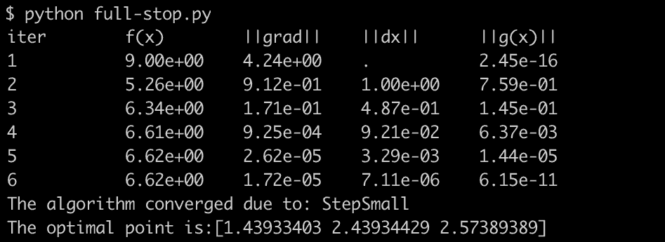
Running the program with inputs $a=2.0$, $\theta_0=0$, $v_0=[2,0]$ and $s=\frac{\pi}{2}$ returns:

The optimal point vector contains the values for $t_s$,$t_a$ and $t_m$. This means that for a ship with the given input, it should start turning immediately, then start the burn after approximately 1.43 seconds, stop turning and only accelerate at 2.43 and finally be at rest after 2.57 seconds, approximately 0.43 seconds faster then the naive version.

To test the result, I implemented a quick and dirty javascript program that simulates these choices and renders to a canvas:

Sometimes the ships end up drifting a bit after the simulation has finished. This is due to the discrete nature of the simulation not perfectly emulating the continuous solution (I do not integrate rotation analytically in the simulation). This could also have been a problem if I applied this style of planning to a game that did the same, from the simulation above it looks negligible though, which is great!

I am very happy with this result, it seems like it could work for the larger problem as well. The next step I’ll try, is to tackle some specific cases of moving from point A to B efficiently. For those cases there will be many more time variables involved, and possibly many constellations of safe initial starting points as well as possible freedoms to introduce in the model. It will be interesting to see how that works out.

Lately I have been looking for a solid way to create a robust implementation moving a spaceship from one point to another. This turned out to be a hard problem, and led me to a lot of new literature, which included Steven M. LaValle’s Planning Algorithms. Randomly reading from it I found a small gem called the van der Corput sequence.

The van der Corput sequence is useful for sampling in an interval. LaValle discusses it as an option to random sampling within the context of sampling for planning algorithms. I had thought about similar issues in the context of root finding, where I always wondered how to predictably generate a sequence that would distribute samples evenly over an interval, as well as do so in a manner that would not “favor” parts of the interval over others.

One naive way to sample over an interval, is to split the interval in X pieces and do the samples in order. If X is 8 and this method is used the interval would be explored as shown to the left in the figure below (clearly this means the the early parts of the interval will be explored first). Using the van der Corput sequence would result in exploration as seen on the right (which explores the interval much more evenly).

Generating the van der Corput sequence is surprisingly simple and elegant, just flip the bits of the naive sequence as seen in the binary column above. I find this very peculiar, since mirrored donkeys do not normally turn into cheetahs.

The great properties of this sequence is that whenever you end it, it will have explored the interval pretty evenly. A second nice property is that you can easily continue the sequence beyond an initial size, by creating the naive sequence at the position you want to start from, and keep reversing the results.

This method will definitely go into my toolbox of things to consider whenever I am thinking about using random sampling.

Tag: Planning

One way to stop a 2D spaceship as fast as possible.

The van der Corput sequence